tfruns: Track and Visualize Training Runs
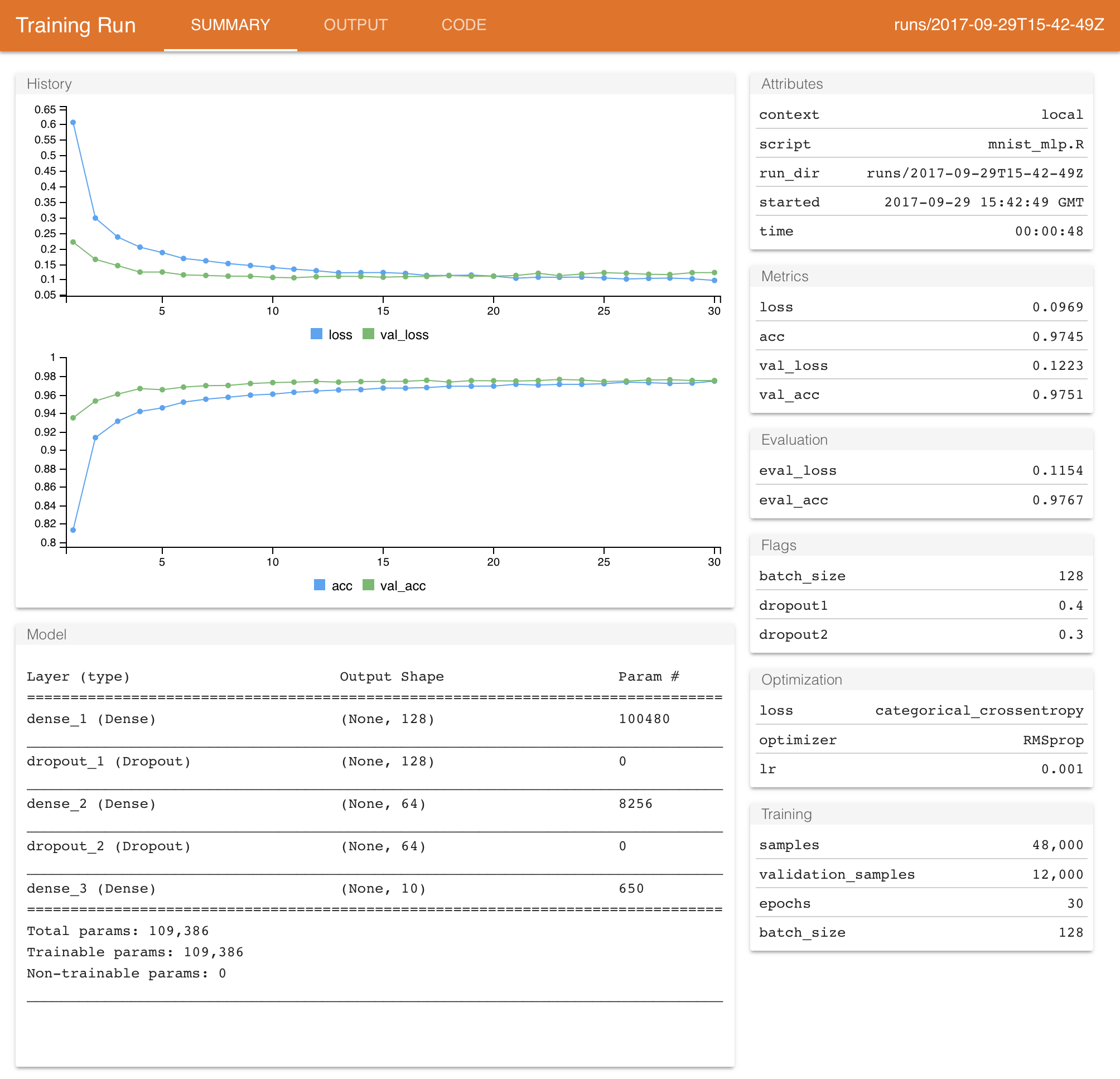
The tfruns package provides a suite of tools for tracking, visualizing, and managing TensorFlow training runs and experiments from R:
Track the hyperparameters, metrics, output, and source code of every training run.
Compare hyperparmaeters and metrics across runs to find the best performing model.
Automatically generate reports to visualize individual training runs or comparisons between runs.
No changes to source code required (run data is automatically captured for all Keras and TF Estimator models).
Installation
You can install the tfruns package from GitHub as follows:
devtools::install_github("rstudio/tfruns")The package is intended to be used with the keras and/or the tfestimators packages, both of which provide higher level interfaces to TensorFlow from R. These packages can be installed with:
install.packages("keras")
install.packages("tfestimators")
Training
In the following sections we’ll describe the various capabilities of tfruns. Our example training script (mnist_mlp.R) trains a Keras model to recognize MNIST digits.
To train a model with tfruns, just use the training_run() function in place of the source() function to execute your R script. For example:
library(tfruns)
training_run("mnist_mlp.R")
When training is completed, a summary of the run will automatically be displayed if you are within an interactive R session:

The metrics and output of each run are automatically captured within a run directory which is unique for each run that you initiate. Note that for Keras and TF Estimator models this data is captured automatically (no changes to your source code are required).
You can call the latest_run() function to view the results of the last run (including the path to the run directory which stores all of the run’s output):
$ run_dir           : chr "runs/2017-10-02T14-23-38Z"
$ eval_loss         : num 0.0956
$ eval_acc          : num 0.98
$ metric_loss       : num 0.0624
$ metric_acc        : num 0.984
$ metric_val_loss   : num 0.0962
$ metric_val_acc    : num 0.98
$ flag_dropout1     : num 0.4
$ flag_dropout2     : num 0.3
$ samples           : int 48000
$ validation_samples: int 12000
$ batch_size        : int 128
$ epochs            : int 20
$ epochs_completed  : int 20
$ metrics           : chr "(metrics data frame)"
$ model             : chr "(model summary)"
$ loss_function     : chr "categorical_crossentropy"
$ optimizer         : chr "RMSprop"
$ learning_rate     : num 0.001
$ script            : chr "mnist_mlp.R"
$ start             : POSIXct[1:1], format: "2017-10-02 14:23:38"
$ end               : POSIXct[1:1], format: "2017-10-02 14:24:24"
$ completed         : logi TRUE
$ output            : chr "(script ouptut)"
$ source_code       : chr "(source archive)"
$ context           : chr "local"
$ type              : chr "training"
The run directory used in the example above is “runs/2017-10-02T14-23-38Z”. Run directories are by default generated within the “runs” subdirectory of the current working directory, and use a timestamp as the name of the run directory. You can view the report for any given run using the view_run() function:
view_run("runs/2017-10-02T14-23-38Z")Comparing Runs
Let’s make a couple of changes to our training script to see if we can improve model performance. We’ll change the number of units in our first dense layer to 128, change the learning_rate from 0.001 to 0.003 and run 30 rather than 20 epochs. After making these changes to the source code we re-run the script using training_run() as before:
training_run("mnist_mlp.R")This will also show us a report summarizing the results of the run, but what we are really interested in is a comparison between this run and the previous one. We can view a comparison via the compare_runs() function:
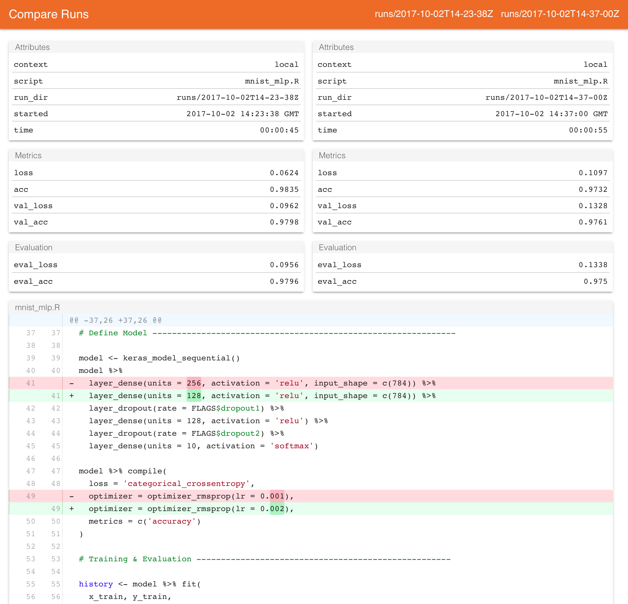
The comparison report shows the model attributes and metrics side-by-side, as well as differences in the source code and output of the training script.
Note that compare_runs() will by default compare the last two runs, however you can pass any two run directories you like to be compared.
Analyzing Runs
We’ve demonstrated visualizing and comparing one or two runs, however as you accumulate more runs you’ll generally want to analyze and compare runs many runs. You can use the ls_runs() function to yield a data frame with summary information on all of the runs you’ve conducted within a given directory:
ls_runs()Data frame: 4 x 28
run_dir eval_loss eval_acc metric_loss metric_acc metric_val_loss metric_val_acc
1 runs/2017-12-09T21-01-11Z 0.1485 0.9562 0.2577 0.9240 0.1482 0.9545
2 runs/2017-12-09T21-00-11Z 0.1438 0.9573 0.2655 0.9208 0.1505 0.9559
3 runs/2017-12-09T19-59-44Z 0.1407 0.9580 0.2597 0.9241 0.1402 0.9578
4 runs/2017-12-09T19-56-48Z 0.1437 0.9555 0.2610 0.9227 0.1459 0.9551
# ... with 21 more columns:
# flag_batch_size, flag_dropout1, flag_dropout2, samples, validation_samples, batch_size,
# epochs, epochs_completed, metrics, model, loss_function, optimizer, learning_rate, script,
# start, end, completed, output, source_code, context, typeYou can also render a sortable, filterable version all of the columns within RStudio using the View() function:
View(ls_runs())
The ls_runs() function also supports subset and order arguments. For example, the following will yield all runs with an eval accuracy better than 0.98:
ls_runs(eval_acc > 0.9570, order = eval_acc)Data frame: 2 x 28
run_dir eval_acc eval_loss metric_loss metric_acc metric_val_loss metric_val_acc
1 runs/2017-12-09T19-59-44Z 0.9580 0.1407 0.2597 0.9241 0.1402 0.9578
2 runs/2017-12-09T21-00-11Z 0.9573 0.1438 0.2655 0.9208 0.1505 0.9559
# ... with 21 more columns:
# flag_batch_size, flag_dropout1, flag_dropout2, samples, validation_samples, batch_size,
# epochs, epochs_completed, metrics, model, loss_function, optimizer, learning_rate, script,
# start, end, completed, output, source_code, context, typeYou can pass the results of ls_runs() to compare runs (which will always compare the first two runs passed). For example, this will compare the two runs that performed best in terms of evaluation accuracy:
compare_runs(ls_runs(eval_acc > 0.9570, order = eval_acc))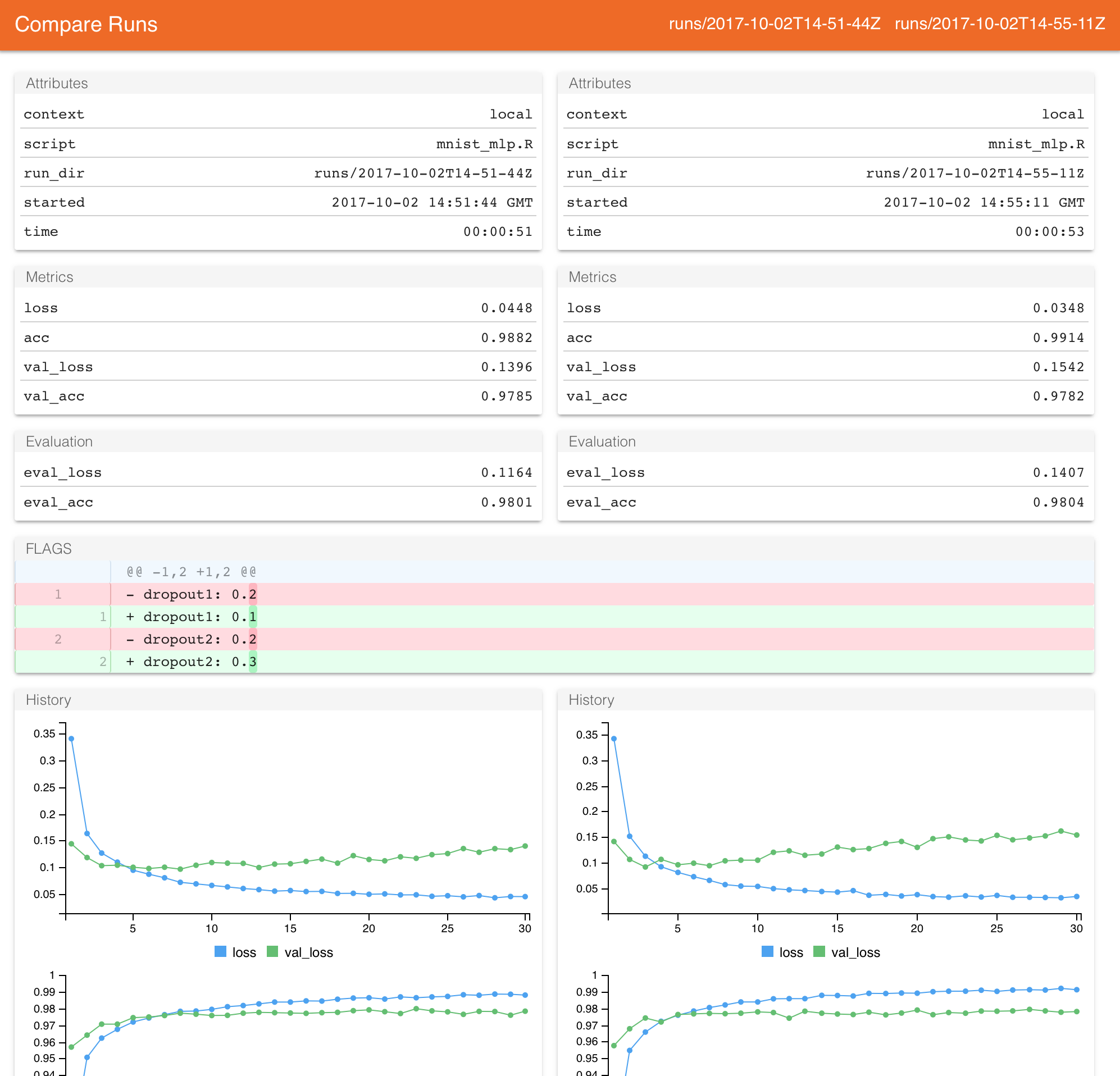
RStudio IDE
If you use RStudio with tfruns, it’s strongly recommended that you update to the current Preview Release of RStudio v1.1, as there are are a number of points of integration with the IDE that require this newer release.
Addin
The tfruns package installs an RStudio IDE addin which provides quick access to frequently used functions from the Addins menu:
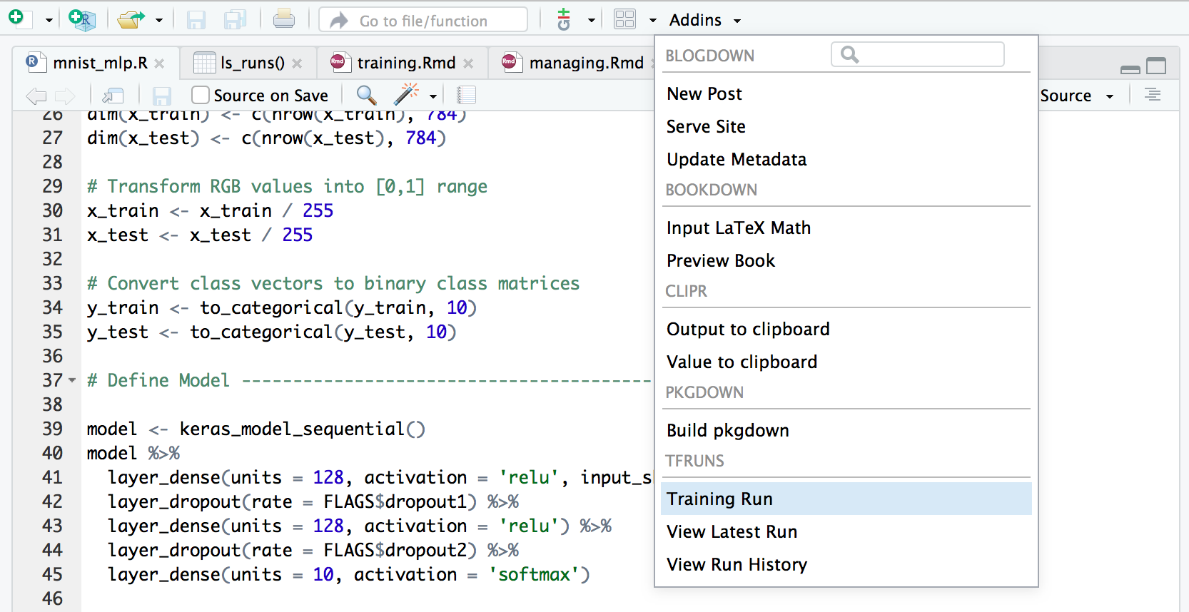
Note that you can use Tools -> Modify Keyboard Shortcuts within RStudio to assign a keyboard shortcut to one or more of the addin commands.
Background Training
RStudio v1.1 includes a Terminal pane alongside the Console pane. Since training runs can become quite lengthy, it’s often useful to run them in the background in order to keep the R console free for other work. You can do this from a Terminal as follows:
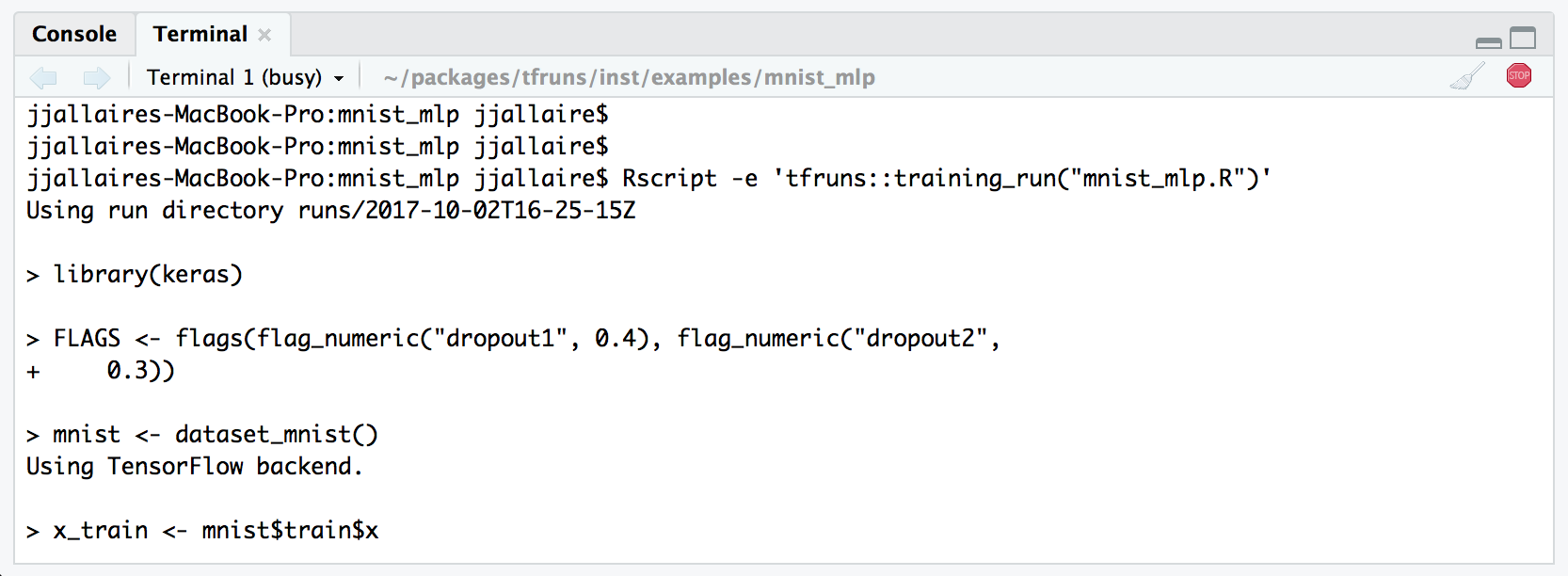
If you are not running within RStudio then you can of course use a system terminal window for background training.
Publishing Reports
Training run views and comparisons are HTML documents which can be saved and shared with others. When viewing a report within RStudio v1.1 you can save a copy of the report or publish it to RPubs or RStudio Connect:
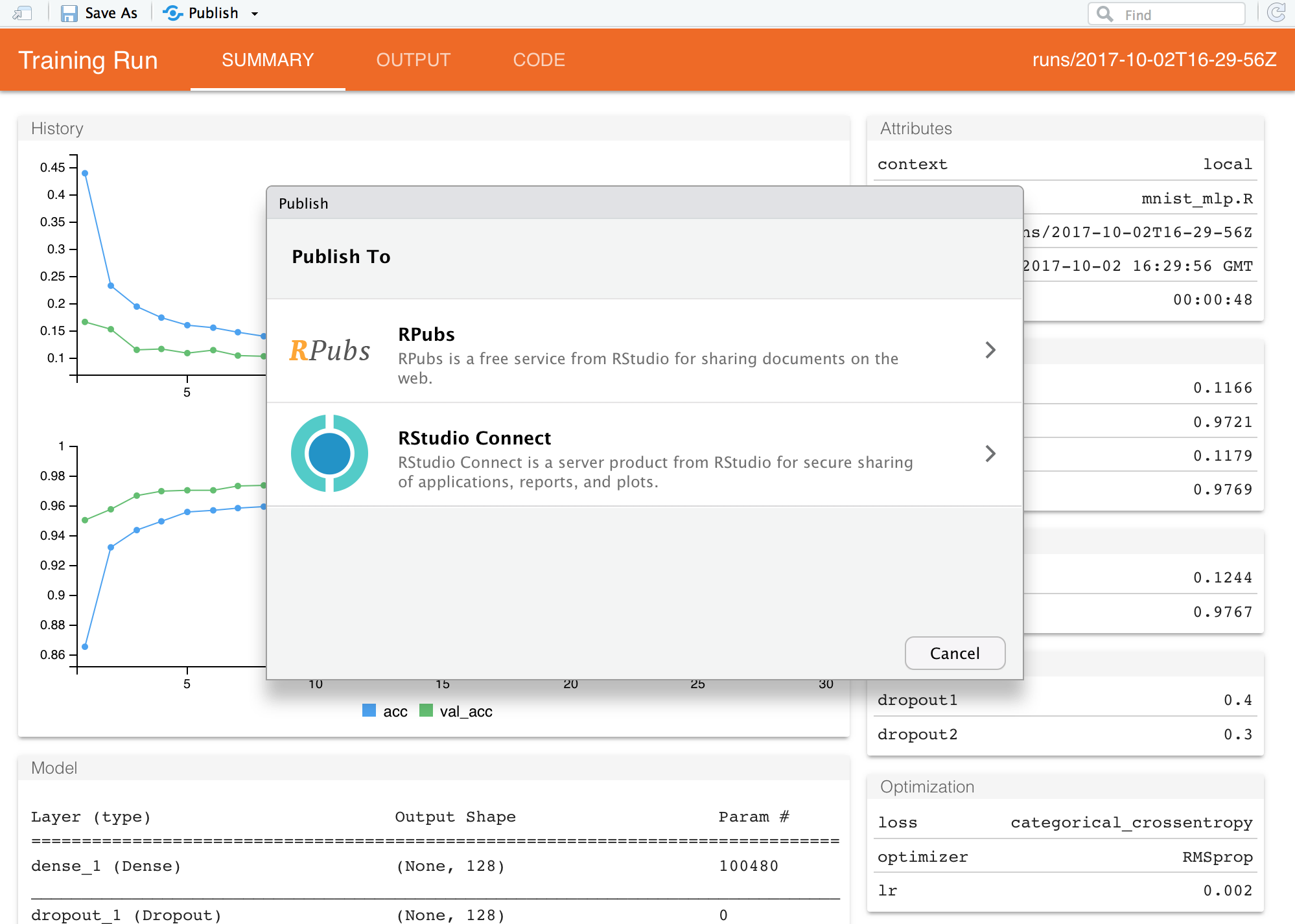
If you are not running within RStudio then you can use the save_run_view() and save_run_comparison() functions to create standalone HTML versions of run reports.
Hyperparameter Tuning
Tuning a model often requires exploring the impact of changes to many hyperparameters. The best way to approach this is generally to systematically train over the combinations of those parameters to determine which combination yields the best model. See the Hyperparmeter Tuning article for details on how to accomplish this with tfruns.
Managing Runs
There are a variety of tools available for managing training run output, including:
Exporting run artifacts (e.g. saved models).
Copying and purging run directories.
Using a custom run directory for an experiment or other set of related runs.
The Managing Runs article provides additional details on using these features.