Training with CloudML
Overview
Training models with CloudML uses the following workflow:
Develop and test an R training script locally
Submit a job to CloudML to execute your script in the cloud
Monitor and collect the results of the job
Tune your model based on the results and repeat training as necessary
CloudML is a managed service where you pay only for the hardware resources that you use. Prices vary depending on configuration (e.g. CPU vs. GPU vs. multiple GPUs). See https://cloud.google.com/ml-engine/pricing for additional details.
Local Development
Working on a CloudML project always begins with developing a training script that runs on your local machine. This will typically involve using one of these packages:
keras — A high-level interface for neural networks, with a focus on enabling fast experimentation.
tfestimators — High-level implementations of common model types such as regressors and classifiers.
tensorflow — Lower-level interface that provides full access to the TensorFlow computational graph.
There are no special requirements for your training script, however there are a couple of things to keep in mind:
When you train a model on CloudML all of the files in the current working directory are uploaded. Therefore, your training script should be within the current working directory and references to other scripts, data files, etc. should be relative to the current working directory. The most straightforward way to organize your work on a CloudML application is to use an RStudio Project.
Your training data may be contained within the working directory, or it may be located within Google Cloud Storage. If your training data is large and/or located in cloud storage, the most straightforward workflow for development is to use a local subsample of your data. See the article on Google Cloud Storage for a detailed example of using distinct data for local and CloudML execution contexts, as well as reading data from Google Cloud Storage buckets.
Once your script is working the way you expect you are ready to submit it as a job to CloudML.
Submitting Jobs
The core unit of work in CloudML is a job. A job consists of a training script and related files (e.g. other scripts, data files, etc. within the working directory). To submit a job to CloudML you use the cloudml_train() function, passing it the name of the training script to run. For example:
library(cloudml)
job <- cloudml_train("mnist_mlp.R")
Note that the very first time you submit a job to CloudML the various packages required to run your script will be compiled from source. This will make the execution time of the job considerably longer that you might expect. It’s only the first job that incurs this overhead though (since the package installations are cached), and subsequent jobs will run more quickly.
The cloudml_train() function returns a job object. This is a reference to the training job which you can use later to check it’s status, collect it’s output, etc. For example:
job_status(job) $ createTime : chr "2017-12-18T20:35:21Z"
$ etag : chr "2KRqIbAhzvM="
$ jobId : chr "cloudml_2017_12_18_203510175"
$ startTime : chr "2017-12-18T20:35:52Z"
$ state : chr "RUNNING"
$ trainingInput :List of 3
..$ jobDir : chr "gs://cedar-card-791/r-cloudml/staging"
..$ region : chr "us-central1"
..$ runtimeVersion: chr "1.4"
$ trainingOutput:List of 1
..$ consumedMLUnits: num 0.04
View job in the Cloud Console at:
https://console.cloud.google.com/ml/jobs/cloudml_2017_12_18_203510175?project=cedar-card-791
View logs at:
https://console.cloud.google.com/logs?resource=ml.googleapis.com%2Fjob_id%2Fcloudml_2017_12_18_203510175&project=cedar-card-791To interact with jobs you don’t need the job object returned from cloudml_train(). If you call job_status() or with no arguments it will act on the most recently submitted job:
job_status() # get status of last jobCollecting Job Results
You can call job_collect() at any time to download a job:
job_collect()     # collect last job
job_collect(job)  # collect specific job
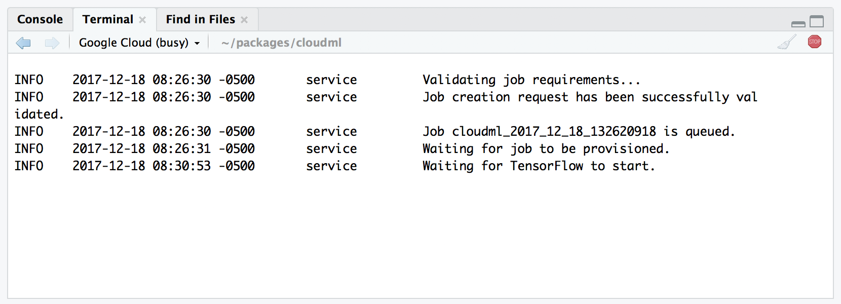
Note also that if you are using RStudio v1.1 or higher you’ll be given the to monitor and collect submitted jobs in the background using an RStudio terminal:

In this case you don’t need to call job_collect() explicitly as this will be done from within the background terminal after the job completes.
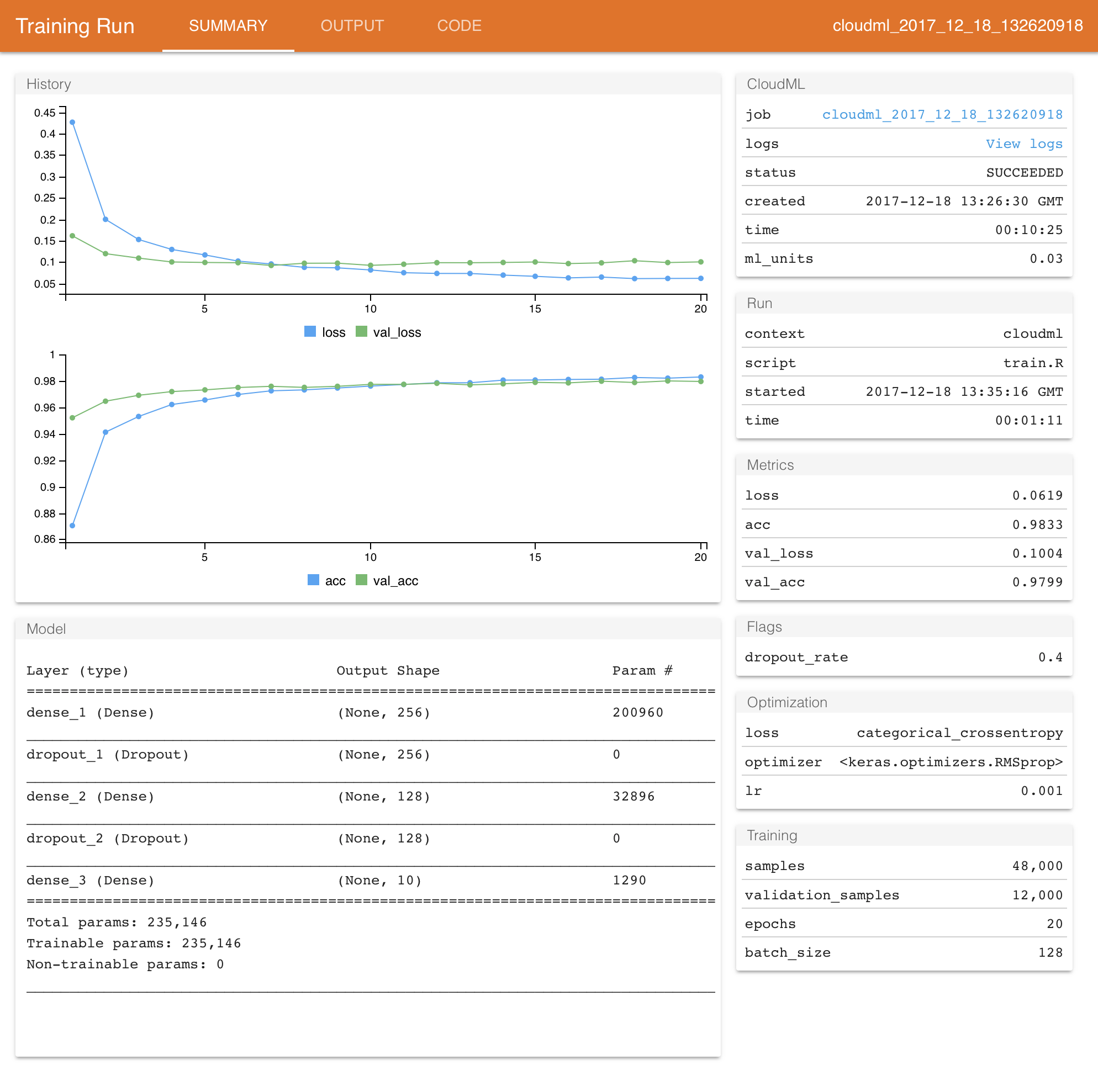
Once the job is complete it’s results will be downloaded and a report will be automatically displayed:

Training Runs
Each training job will produce one or more training runs (it’s typically only a single run, however when doing hyperparmeter turning there will be multiple runs). When you collect a job from CloudML it is automatically downloaded into the runs sub-directory of the current working directory.
You can list all of the runs as a data frame using the ls_runs() function:
ls_runs()Data frame: 6 x 37
run_dir eval_loss eval_acc metric_loss metric_acc metric_val_loss metric_val_acc
6 runs/cloudml_2018_01_26_135812740 0.1049 0.9789 0.0852 0.9760 0.1093 0.9770
2 runs/cloudml_2018_01_26_140015601 0.1402 0.9664 0.1708 0.9517 0.1379 0.9687
5 runs/cloudml_2018_01_26_135848817 0.1159 0.9793 0.0378 0.9887 0.1130 0.9792
3 runs/cloudml_2018_01_26_135936130 0.0963 0.9780 0.0701 0.9792 0.0969 0.9790
1 runs/cloudml_2018_01_26_140045584 0.1486 0.9682 0.1860 0.9504 0.1453 0.9693
4 runs/cloudml_2018_01_26_135912819 0.1141 0.9759 0.1272 0.9655 0.1087 0.9762
# ... with 30 more columns:
# flag_dense_units1, flag_dropout1, flag_dense_units2, flag_dropout2, samples, validation_samples,
# batch_size, epochs, epochs_completed, metrics, model, loss_function, optimizer, learning_rate,
# script, start, end, completed, output, source_code, context, type, cloudml_console_url,
# cloudml_created, cloudml_end, cloudml_job, cloudml_log_url, cloudml_ml_units, cloudml_start,
# cloudml_stateYou can view run reports using the view_run() function:
# view the latest run
view_run()

# view a specific run
view_run("runs/cloudml_2017_12_15_182614794")
There are many tools available to list, filter, and compare training runs. For additional information see the documentation for the tfruns package.
Managing Jobs
You can enumerate previously submitted jobs using the job_list() function:
job_list() JOB_ID STATUS CREATED
1 cloudml_2017_12_18_203510175 SUCCEEDED 2017-12-18 15:35:21
2 cloudml_2017_12_18_202228264 FAILED 2017-12-18 15:22:39
3 cloudml_2017_12_18_201607948 SUCCEEDED 2017-12-18 15:16:18
4 cloudml_2017_12_18_132620918 SUCCEEDED 2017-12-18 08:26:30
5 cloudml_2017_12_15_182614794 SUCCEEDED 2017-12-15 13:26:29
6 cloudml_2017_12_14_183247626 SUCCEEDED 2017-12-14 13:33:04You can use the JOB_ID field to interact with any of these jobs:
job_status("cloudml_2017_12_18_203510175")The job_stream_logs() function can be used to view the live log of a running job:
job_stream_logs("cloudml_2017_12_18_203510175")The job_cancel() function can be used to cancel a running job:
job_cancel("cloudml_2017_12_18_203510175")Tuning Your Application
Tuning your application typically requires choosing and then optimizing a set of hyperparameters that influence your model’s performance. This could include the number and type of layers, units within layers, drop rates, regularization, etc.
You can experiment with hyperparameters on an ad-hoc basis, but in general it’s better to explore them more systematnically. The key to doing this with CloudML is by defining training flags within your script and the parameterizing runs using those flags.
For example, you might define the following training flags:
library(keras)

FLAGS <- flags(
  flag_integer("dense_units1", 128),
  flag_numeric("dropout1", 0.4),
  flag_integer("dense_units2", 128),
  flag_numeric("dropout2", 0.3),
)
Then use the flags in a script as follows:
input <- layer_input(shape = c(784))
predictions <- input %>%
  layer_dense(units = FLAGS$dense_units1, activation = 'relu') %>%
  layer_dropout(rate = FLAGS$dropout1) %>%
  layer_dense(units = FLAGS$dense_units2, activation = 'relu') %>%
  layer_dropout(rate = FLAGS$dropout2) %>%
  layer_dense(units = 10, activation = 'softmax')

model <- keras_model(input, predictions) %>% compile(
  loss = 'categorical_crossentropy',
  optimizer = optimizer_rmsprop(lr = 0.001),
  metrics = c('accuracy')
)

history <- model %>% fit(
  x_train, y_train,
  batch_size = 128,
  epochs = 30,
  verbose = 1,
  validation_split = 0.2
)
Note that instead of literal values for the various hyperparameters we want to vary we now reference members of the FLAGS list returned from the flags() function.
You can try out different flags by passing a named list of flags to the cloudml_train() function. For example:
cloudml_train("minst_mlp.R", flags = list(dropout1 = 0.3, dropout2 = 0.2))These flags are passed to your script and are also retained as part of the results recorded for the training run.
You can also more systematically try combinations of flags using CloudML hyperparameter tuning.
Training with a GPU
By default, CloudML utilizes “standard” CPU-based instances suitable for training simple models with small to moderate datasets. You can request the use of other machine types, including ones with GPUs, using the master_type parameter of cloudml_train().
For example, the following would train the same model as above but with a Tesla K80 GPU:
cloudml_train("train.R", master_type = "standard_gpu")To train using a Tesla P100 GPU you would specify "standard_p100":
cloudml_train("train.R", master_type = "standard_p100")To train on a machine with 4 Tesla P100 GPU’s you would specify "complex_model_m_p100":
cloudml_train("train.R", master_type = "complex_model_m_p100")See the CloudML website for documentation on available machine types. Also note that GPU instances can be considerably more expensive that CPU ones! See the documentation on CloudML Pricing for details.
Training Configuration
You can provide custom configuration for training by creating a cloudml.yml file within the working directory from which you submit your training job. This file can be used to customize various aspects of training behavior including the virtual machines used as well as the runtime version of CloudML used in the job.
For example, the following config file specifies a custom scale tier with a master type of “large_model”. It also specifies that the CloudML runtime version should be 1.2.
cloudml.yml
trainingInput:
  scaleTier: CUSTOM
  masterType: large_model
  runtimeVersion: 1.2
You can also pass a named configuration file (i.e. one for a hyperparameter tuning job) via the config parmater of cloudml_train(). For example:
cloudml_train("mnist_mlp.R", config = "tuning.yml")Note that trainingInput is used as the top level key in the config file (this is required). Additional documentation on available fields in the configuration file is available here https://cloud.google.com/ml-engine/reference/rest/v1/projects.jobs#TrainingInput.
Learning More
The following articles provide additional documentation on training and deploying models with CloudML:
Hyperparameter Tuning explores how you can improve the performance of your models by running many trials with distinct hyperparameters (e.g. number and size of layers) to determine their optimal values.
Google Cloud Storage provides information on copying data between your local machine and Google Storage and also describes how to use data within Google Storage during training.
Deploying Models describes how to deploy trained models and generate predictions from them.